Writing a SIMD Raytracer

A Meal of Many Courses

This is the first part of a short series of articles about fast raytracing on the CPU. The first article covers the background as well as the raytracer architecture, while followup instalments will focus on various technical and mathematical bits, such as SIMD intersection math, SAH optimization, putting multiple SIMD backends in one binary, threading, memory allocation, and so on.

Because we are going to be focusing on fast for most of the article, there will be assumptions of raytracing, math, programming and computer knowledge. To not leave people behind, I'll explain some basics as we go, but to get deeper understanding, I wholeheartedly recommend doing your own research. A good place to start is the Raytracing Weekend book series. For computer knowledge (virtual memory, cache lines, SIMD), my long-form recommendation for the patient viewer is Casey Muratori's Handmade Hero and Computer Enhance series.

If you already know all this and want to skip over to "the good part", you can go to the section Raytracer Architecture, Second Main Course.

The article stems from work I did in early 2023. As of the time of writing (December 2025), that work is still the most focused nugget of technical work I have done. This was quite the luxury for me as I usually don't get to concentrate on doing single part of a larger system well, and instead have to prioritize what is the most valuable thing to work on. A happy and rare exception.

Now, before we get to the core of the problem, here's the last bit of context. In early 2023, a startup company I worked for was about to get funding, and we wanted to warm up the programming team on a thing we knew we were going to need before fanning out and developing the rest. The goal of the company was to give real estate developers tools to procedurally generate housing architecture. This housing was supposed to meet the developer's criteria, such as yields, mix of functions and apartment sizes, aesthetics, as well as spatial instructions (e.g. build here but not there, build in this shape...). We assumed that to generate the architecture, there would be a computer learning process. As it is with learning processes, they need to get feedback on their results from one iteration that can be fed into the next, gradually improving the results. Architecture is a very high-dimensional problem space. A house is definitely not just any house shaped geometry, and before we even enter the realm of architecture, there's structural engineering, business, regulatory and legal criteria that a house must satisfy. For such a tall order, we assumed that even a smartly designed learning algorithm will have to do many iterations, getting feedback from a myriad of evaluators (structural, sunlight/daylight, acoustic, business, legal) until it reaches a solution.

So we generate stuff, evaluate, generate new stuff, evaluate, and so on, until eventually we stop after either all criteria are satisfied, no significant improvement can be found, or we exceeded our computational budget. And because the problem is going to be hard, we need to use that budget well. At the time we weren't quite sure whether we need to be fast so that we have a shot at being quasi-realtime, or to at least finish the computation overnight on a powerful hardware [1].

The thing we focused on first was one particularly computationally demanding part of the evaluation process: the daylight evaluation. For the uninitiated, it is something that tells you how much light accumulates on surfaces in the interior of a building for some stable lighting conditions outside. This is done for up to tens of thousands of surfaces inside many rooms and many buildings in a city block, both in the buildings you plan to build, and in the already existing buildings that surround them [2].

The way daylight evaluation is usually implemented today is raytracing. Interestingly enough, all software solutions that existed in 2023 (Ladybug, Climate Studio) internally depend on a raytracing package called Radiance. For various reasons, both Radiance itself and the way it is integrated into products is a few orders of magnitude too slow to be useful as a machine learning feedback function, or a human design feedback function, for that matter [3]. We believed those orders of magnitude could be reclaimed, and thus our first quest was to build a fast daylight evaluator for our internal use [4].

Ray Tracing

To bridge this closer to videogame audience, daylight evaluation is very similar to what game developers call light baking: computing light simulation for static scenes and baking the results into planar (lightmaps) or spatial (light probes) textures, so that we know how a scene is lit without having to compute it at runtime. The differences between daylight evaluation and light baking come down to how the results are used, not how they are computed. Compared to light baking, daylight evaluation doesn't care about color, only intensity, nor does it need to produce information about which direction the light is coming from for the light probes. Daylighting also only needs to simulate perfectly diffuse (Lambertian) materials, making some parts of the job simpler. There's also a few peripheral bits about interpreting the results that are specific to the AEC industry. I am going to purposefully ignore these, and instead focus on raytracing, which I believe looks the same as it would in a computer graphics application.

Ray tracing is a process of simulating light. For a point in space, for instance a pixel on a chip of a digital camera, we want to determine the intensity and color of light that point receives. We do that by simulating paths that light could have taken through the scene from a light source to reach our point. Such paths can be either direct, or include one or more bounces from objects in the scene. However, we are often interested in light reaching just a few select points in space, like the chip of our digital camera. Compared to all the places the light can go, light rays have only a miniscule chance of reaching the points we are interested in, directly or via bounces. In other words, we would have to shoot a lot of rays from light sources for them to trickle down to our measurement points in sufficient quantities.

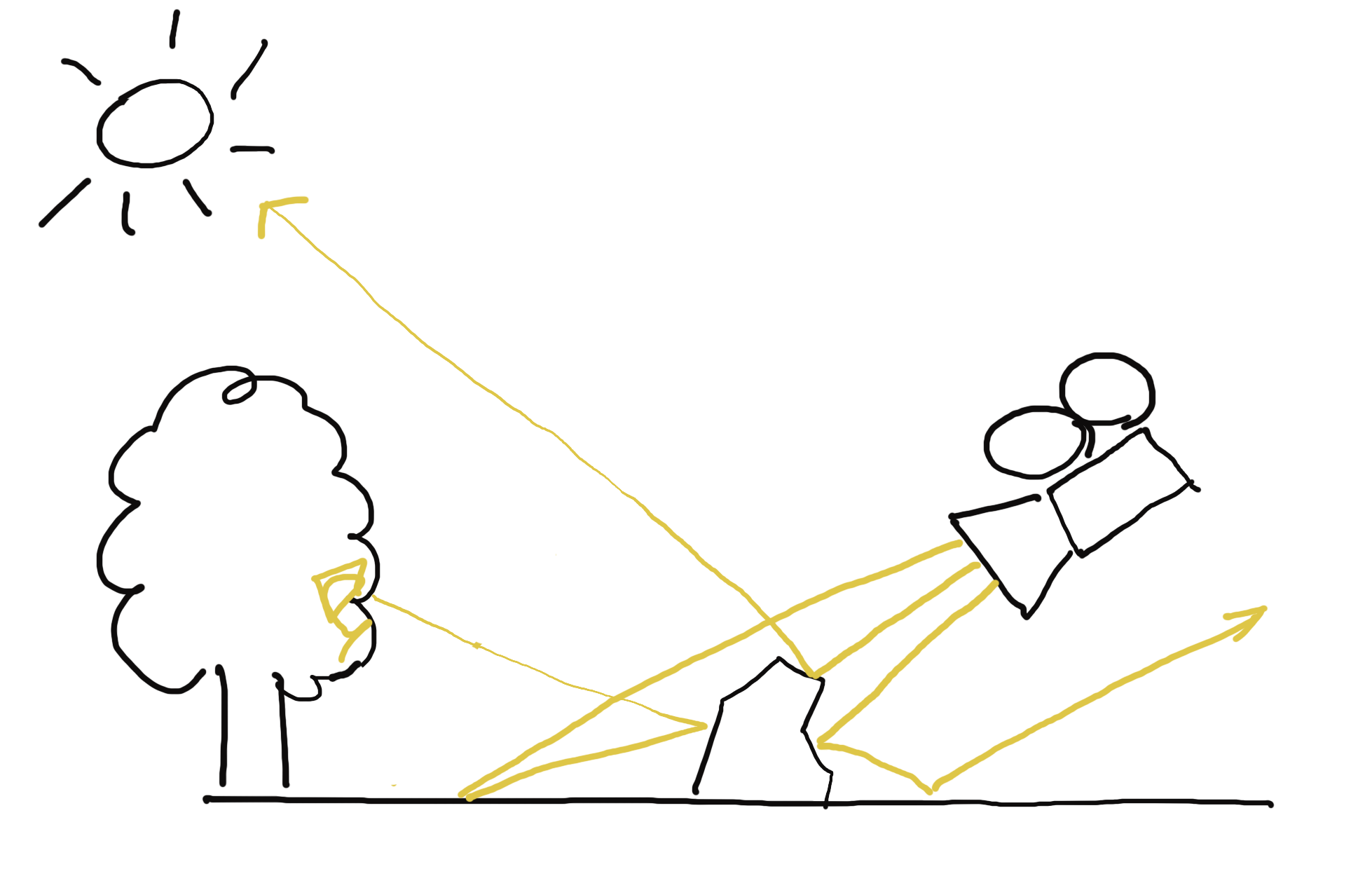
Instead, we lean on laws of the universe regarding (the absence of) the arrow of time for the behavior of particles. If we were shown a movie of elementary particles moving through space, perhaps sometimes colliding with each other, we would have a hard time telling, whether the movie is playing forward or backward. This is because it is impossible to tell - they follow the same rules whether they are moving forward or backward in time, and it is only possible to discern the direction of time once we have a large number of particles and probability enters the picture, pushing particles towards states with high entropy [5]. For us, this means that if we have a path between a measurement point and a light source, a photon could have taken that exact path in both directions [6].

The implication of bidirectionality for our simulation is that we can trace rays in reverse: from the relatively few points we are interested in towards light sources. For infinite number of rays we would have reached the same answer either way, but with our finite limitations, we have a higher chance of successfully completing the path between the light source and the camera going backwards [7]. With both forward and reverse raytracing, we keep track of how much energy we lose each bounce. Because these energy losses (also called attenuation) multiply, and multiplication is commutative, this works out the same regardless of the direction we trace the ray in.

So we trace rays from our measurement points, hoping they eventually reach sources of light. These rays go in a straight line until they hit something. Depending on what was hit, various things happen.

If the ray hits a light reflecting surface, it bounces off of it, back into the scene. The new direction of the ray depends on the physical properties of the surface. Some surfaces reflect the ray as a mirror would, others deflect the ray in a random direction, and there are more complicated behaviors for realistic materials, described by the material's Bidirectional Reflectance Distribution Function (BRDF). A BRDF can be quite complex [8], and cannot always be defined by a mathematical formula. For many realistic materials, the BRDF is actually a lookup table [9], measured by putting the material in a Gonioreflectometer.

If the ray hits a light source, it ends its journey. We read the light's value and apply the attenuation the ray has accumulated when bouncing off of materials along its path. Because each bounce attenuates the ray, we also can decide to terminate the ray early after a certain amount of bounces, because even if it did reach a light source eventually, the light's contribution through that particular ray would have been close to zero.

Hopefully multiple rays shot from our camera reach light sources. We compute the light value reaching the camera's pixel as the sum of individual ray contributions divided by the number of cast rays. Because scenes are not always well lit, it may take a lot of rays for us to form a coherent picture of what the scene looks like from the perspective of the camera. Low light scenes are prone to noise, when various neighboring pixels in the camera collect dramatically different values of light due to randomness of bounces. As the number of rays increases to infinity, the noise becomes weaker, but because a large number of rays is not always practical, we often employ denoising algorithms that reconstruct information from noisy pictures. Denoising is an important part of modern raytracing, because it lets us spend a fixed cost to substantially improve the result quality that would otherwise have to be improved by shooting unreasonable amounts of rays. It might have also been useful in our usecase [10], but we simply didn't have the time to pursue it.

Raytracer Architecture, Appetizer

At a high level, a raytracer operates on a geometric description of the scene and a list of rays it needs to compute on that scene. These do not necessarily change at the same rate from frame to frame, and many real-time raytracers reason about that (but we won't).

The simplest and most flexible way to represent the scene is to have arrays of various geometric primitives: triangles, spheres, planes, boxes... Raytracing the scene is about going over each ray and testing [11] it against all of these arrays, remembering information about the closest hit, so that we know where to start our next bounce. In fact, this is so simple that almost all of it fits in pseudocode.

Before addressing the elephant in the room and moving on from this approach, I want to mention some of its benefits.

Firstly, this code listing is almost all there is to it! You have the arrays of objects, and you loop over them. Or, if you don't have data in the exact right shape, you can organize it into those arrays easily. This is not going to be true for the later, more sophisticated designs. There is beauty in simplicity.

Another virtue of the scene laid out in arrays is that the resulting code is very straightforward to optimize. We can easily start thinking about packing the arrays such that each cache line of geometry we load is not going to be wasted [12].

We can also quite easily make the code SIMD [13]. Going wide can happen either over rays or geometries. When going wide over rays, we not only get the obvious benefit of testing multiple rays against geometry, but there is also a subtler compounding effect: we get a lot more value out of each geometry we load, because we test it against multiple rays at a time. Problems arise with some rays finishing after less bounces than others, making the contents of our wide registers be both active and finished rays. We either have to do something about that [14], or accept the wasted work. Going wide over rays was the route taken by Casey Muratori in his Handmade Ray educational miniseries.

Unlike parallelizing on rays, going wide over geometry doesn't ameliorate the cost of memory traffic to the CPU. Each wide geometric primitive is loaded to be tested against a ray, evicted by subsequent loads [15], only to be loaded again when the next ray is going to need that exact same memory. It still is an improvement over the non-SIMD version, as we at least compute more intersections at a time. It is also simpler to think about (unless you think about SIMD a lot), because the nature of the code is still mostly scalar and you only do SIMD to accelerate select parts.

Now back to the elephant, which is algorithmic in nature. We are visiting each geometry for each ray bounce, but most of those rays have no way to reach most geometries. This incurs many wasted loads and calculations per bounce. To get away from the O(m*n), we use acceleration structures to help with eliminating impossible hits, such as Bounding Volume Hierarchies (BVH) or Octrees. Choosing a datastructure depends on the character of your data. We went with the BVH, because it doesn't have many assumptions and degrades gracefully with bad quality of input [16].

Raytracer Architecture, Main Course

The BVH is a tree where each node has a bounding volume geometrically containing the node's contents. This bounding volume is usually a parametric shape, such as an axis-aligned box or a sphere. The node's contents are either links to child nodes, or in case of leaf nodes actual geometries. Note that a node's bounding volume only has a relation to the node's contents, but there is no direct relation between the bounding volumes of two sibling tree nodes. Two sibling nodes can very well have overlapping bounding volumes, both of which are contained inside the parent's bounding volume. This means that a BVH lookup can take multiple paths at the same time, as they aren't necessarily mutually exclusive, unlike in binary search trees.

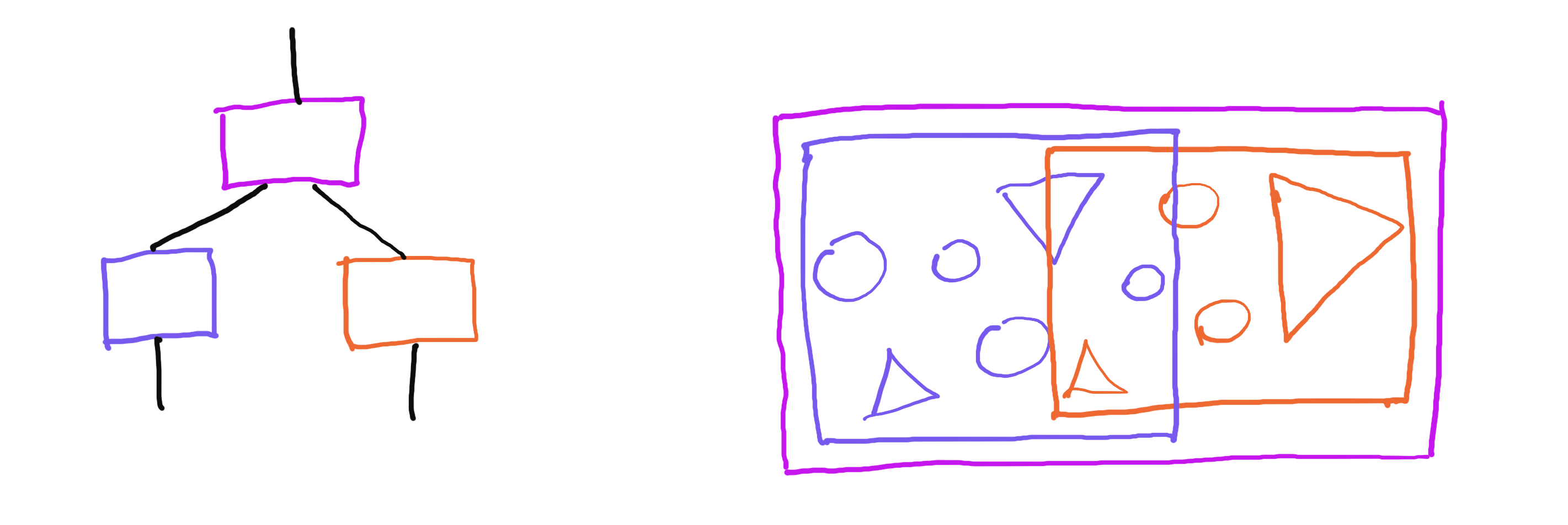
Tree hierarchy (left); Geometry view (right). Note how bounding boxes of the child nodes can overlap, but are contained in the bounding box of the parent node.

In practice, a bounding volume can be any volumetric geometry [17] and the leaf nodes can store whatever we want, but our raytracer used axis-aligned bounding boxes and triangles, so we are going to do the same here.

Testing rays against a BVH is not all that different to what we have been doing until now. We are still going to be keeping track of the closest hit, which is one of the triangles in the leaf nodes. To get to those triangles, we traverse the tree, testing against each node's bounding volume. However, we only visit child nodes, if the ray intersects with the parent node's volume. Once we get to a leaf node, we test our ray against the node's geometry, recording track of the closest hit distance and normal. Once we know the closest hit distance, we can use it to eliminate entire branches of the tree, because we can skip over nodes not just when we miss their bounding volume, but also if the distance to that bounding volume is greater than the recorded closest hit distance. It is worthwhile to traverse the tree depth-first, so that we record our closest hit as soon as possible, eliminating further tests down the line.

Building a BVH is just a little more complicated than using it. I mentioned previously that a node's bounding volume has no relation to bounding volumes of sibling nodes. This makes it a little easier to build a bad-but-correct BVH. For a good BVH, we'd also like to minimize the volume each node takes, and make bounding volumes of sibling nodes overlap less. We'll work on building a good BVH in a future instalment.

Starting with an array of triangles, we begin building the hierarchy by conceptually putting all the triangles into a single BVH node. We then recursively split nodes until the number of triangles they contain is below a predefined threshold.

make_bvh :: (_triangles: [] Triangle) -> BVH {
    bvh: BVH;
    array_add(*bvh.nodes);

    Frame :: struct {
        node_index: s64;
        triangles: [] Triangle;
    }

    stack: [..] Frame;
    array_add(*stack, { 0, _triangles });

    while stack.count {
        frame := pop(*stack);

        node_index := frame.node_index;
        triangles  := frame.triangles;

        node := *bvh.nodes[node_index];

        if triangles.count <= LEAF_TRIANGLE_COUNT {
            node.bbox = aabox_from_triangles(triangles);
            node.type = .LEAF;

            node.leaf.triangle_count = triangles.count;
            array_view_copy(*node.leaf.triangles, triangles, triangles.count);
        } else {
            left_index  := bvh.nodes.count;
            right_index := bvh.nodes.count + 1;

            array_add(*bvh.nodes);
            array_add(*bvh.nodes);

            node.bbox = aabox_from_triangles(triangles);
            node.type = .INNER;

            node.inner.left  = left_index;
            node.inner.right = right_index;

            size_x := node.bbox.max.x - node.bbox.min.x;
            size_y := node.bbox.max.y - node.bbox.min.y;
            size_z := node.bbox.max.z - node.bbox.min.z;

            // Compare one of the triangle points.
            // We could compare centroids instead.
            compare_x :: (a: Triangle, b: Triangle) -> f32 {
                return a.v0.x - b.v0.x;
            }
            compare_y :: (a: Triangle, b: Triangle) -> f32 {
                return a.v0.y - b.v0.y;
            }
            compare_z :: (a: Triangle, b: Triangle) -> f32 {
                return a.v0.z - b.v0.z;
            }

            if size_x > size_y && size_x > size_z {
                quick_sort(triangles, compare_x);
            } else if size_y > size_z {
                quick_sort(triangles, compare_y);
            } else {
                quick_sort(triangles, compare_z);
            }

            left, right := split_array_view(triangles, triangles.count / 2);

            array_add(*stack, { left_index, left });
            array_add(*stack, { right_index, right });
        }
    }

    return bvh;
}
        

Now the raytracer scales logarithmically with the size of the scene. However, by naively entering the land of computer science, we have temporarily lost our ability to utilize modern hardware, and have to do some thinking to recover it.

Raytracer Architecture, Second Main Course

While the raytracer now has good scaling with the size of the scene, we are not utilizing any intra-core parallelism yet, which is a theoretical 4x/8x (perhaps more, if you are reading this in the future) within our reach. Currently, each ray has to traverse the BVH, test against the axis-aligned bounding boxes of its nodes, and for each leaf also test against each triangle, one scalar battle after another.

There's two general avenues of improvement we could explore from here, analogous to the simple array architecture from earlier: parallelizing on rays, or parallelizing on geometry traversal.

Unfortunately, in 2023 I wasn't smart enough to figure out the ray-parallel design that would also include a BVH, and even today I am not sure it would work out all that well. If anyone actually did this, I'd love to know what you did.

Instead we are going to go the obvious way, SIMD crunching multiple geometries against a single ray. While you can readily imagine how we'd SIMD-ify testing rays against triangles in leaf nodes, the more interesting part is applying SIMD to test the bounding volumes. The most obvious challenge here is that the data is not even remotely organized to do this. The bounding boxes are stored in nodes of a binary tree, each node floating who knows where in memory. However, what if we could reshape the tree such that it is essentially the same tree, but the bounding boxes we test against are laid out next to each other?

The transform we are going to do involves changing the tree's branching factor, as well as pulling the child nodes' bounding volumes into the parent node. In some sense, this is the core idea of the raytracer codebase (and this article). At the time I was very happy that I came up with it on my own, but it looks obvious in hindsight. Cursory internet search says other people also do this [18].

However, before we get to the exciting wide BVH, there is one last piece of housekeeping. In the previous version, both types of BVH nodes were stored in a single array and we interpreted their contents based on the type tag.

Since we are about to do SIMD (which arguably means rolling up our sleeves and becoming serious programmers), we would like to leave the heterogeneous tree nodes behind. There's two problems with the union in our nodes, the main one being that it makes it harder to think about the memory we have to load when we walk the tree. We want to make sure that each loaded byte and cache line counts. Towards that end, we would like to have the nodes contain only what we need, align them to cache lines and make sure they do not straddle cache line boundaries. This is not impossible to do for the heterogeneous tree, but at least for me it is simpler to think about it without the overlay. The second problem is memory use. This is not such a big deal today [19], but still it would be nice if we allocated only what we used.

Our new BVH has two kinds of nodes, each stored in their own array. The inner nodes contain indices that point into either inner or leaf nodes. The leaf nodes only contain triangle and material data.

BVH :: struct {
    inner_nodes: [..] Inner_Node;
    leaf_nodes:  [..] Leaf_Node;
}

Inner_Node :: struct {
    bbox: AABox;

    left: BVH_Index;
    right: BVH_Index;
}

Leaf_Node :: struct {
    bbox: AABox;

    count: s64;
    triangles: [LEAF_TRIANGLE_COUNT] Triangle;

    // For now the materials are along for the ride,
    // but we'll store them on a cold cache line soon.
    materials: [LEAF_TRIANGLE_COUNT] Material;
}

// 2:62; 2 bits of tag to select the array, 62 bits to index into the array.
BVH_Index :: struct {
    value: u64;

    TAG_NIL:   u64 : 0; // There is nothing behind indices tagged with NIL.
    TAG_INNER: u64 : 1; // INNER indices point to the inner_nodes array.
    TAG_LEAF:  u64 : 2; // LEAF indices point to the leaf_nodes array.
}

compose_inner_node_index :: (index: s64) -> BVH_Index {
    assert(index < 1 << 62);
    return { (TAG_INNER << 62) | cast(u64, index) };
}

compose_leaf_node_index :: (index: s64) -> BVH_Index {
    assert(index < 1 << 62);
    return { (TAG_LEAF << 62) | cast(u64, index) };
}

decompose_node_index :: (bvh_index: BVH_Index) -> tag: u64, index: s64 {
    MASK: u64 : (1 << 62) - 1;

    tag   := bvh_index.value >> 62;
    index := cast(s64, MASK & bvh_index.value);
    return tag, index;
}
        

Now we are ready to make our BVH wide.

From now on, the code snippets will target AVX hardware (8-wide), because the cache line math works out nicely compared to 4-wide, but we could just as well build SSE/NEON (4-wide) or AVX-512 (16-wide) versions of the data structures. In fact, in one of the followup articles we will talk about how multiple implementations can coexist side by side and produce the same results.

To make the BVH wide, we restructure it slightly. I am going to do so in steps to make it easier to follow. First, imagine the node's bounding volume is not stored in the node itself, but its parent. For the root node, we omit a bounding volume altogether and say it is always reachable.

Inner_Node :: struct {
    left_bbox:  AABox;
    right_bbox: AABox;

    left_index:  BVH_Index;
    right_index: BVH_Index;
}
        

With nodes storing the bounding boxes of their child nodes, we now know whether our ray will hit the child nodes before we visit them. More importantly, the bounding boxes are now stored next to each other, and we could process them both at the same time. In fact, if we stopped here, it is possible that the out-of-order window would be large enough so that the CPU would schedule both intersection tests in parallel.

But why stop at two:

Inner_Node_X8 :: struct {
    child_bbox0: AABox;
    child_bbox1: AABox;
    child_bbox2: AABox;
    child_bbox3: AABox;
    child_bbox4: AABox;
    child_bbox5: AABox;
    child_bbox6: AABox;
    child_bbox7: AABox;

    child_index0: BVH_Index;
    child_index1: BVH_Index;
    child_index2: BVH_Index;
    child_index3: BVH_Index;
    child_index4: BVH_Index;
    child_index5: BVH_Index;
    child_index6: BVH_Index;
    child_index7: BVH_Index;
}
        

Now that all that data is snugly together, all that's left before we vectorize is to align stuff. We might as well factor out the 8-wide axis-aligned box type, since that is what our intersection routine will be operating on. The final version of the wide node:

AABox_Pack_X8 :: struct {
    min: Vec3x8;   #align 64;
    max: Vec3x8;
}

// The node is aligned to the x64 cache line size, and spans 4 cache lines.
Inner_Node_X8 :: struct {
    // Hot, 3 cache lines
    aabox_pack: AABox_Pack_X8;
    // Also likely hot, 1 cache line
    child_indices: [8] BVH_Index;
}
        

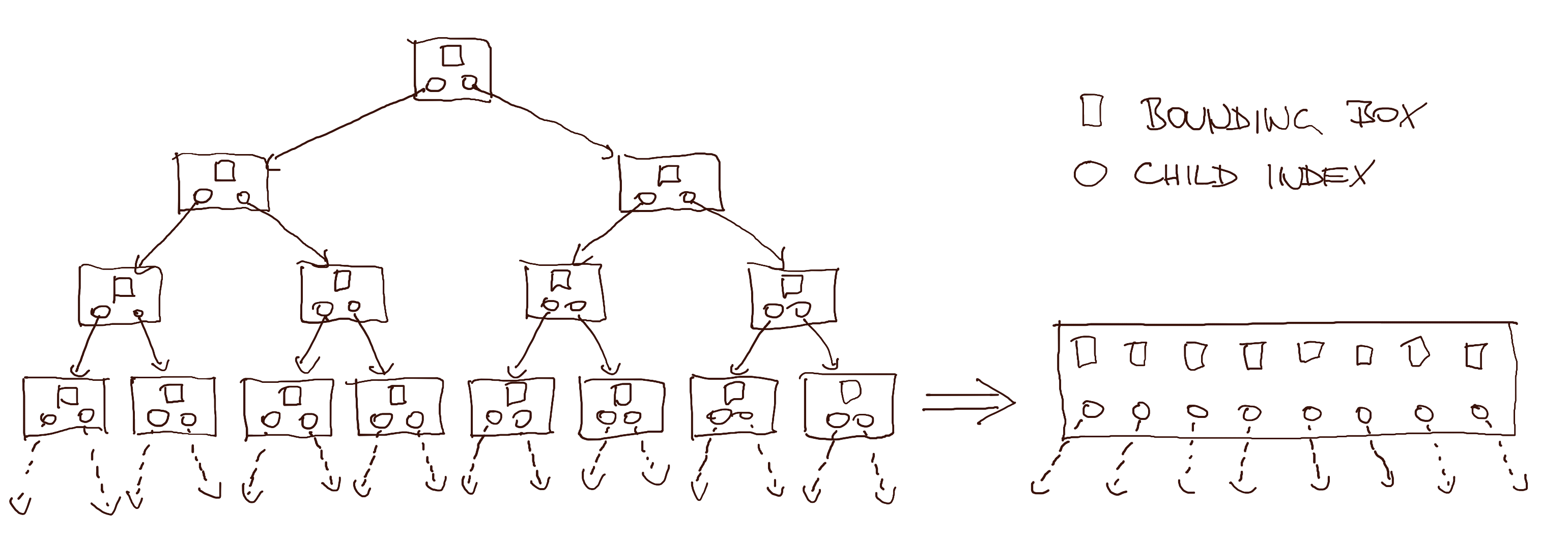
Regular BVH to wide BVH transformation. Wide node on the right has indices from the third row and bounding boxes from the fourth row on the left.

With the 8-wide bounding box, we need a new intersection routine, but the interface is similar to the old one:

Compared to organizing the tree for SIMD, once we crunch through the tree and reach the triangles stored in leaves, going wide is fairly straightforward. One slight subtlety is that instead of triangle count, we are going to have a triangle mask instead, which nicely pads the memory to 5 cache lines. The struct defining the leaf node looks like this:

Leaf_Node_X8 :: struct {
    // Hot, 5 cache lines
    triangle_pack: Triangle_Pack_X8;
    triangle_mask: u32x8;

    // Cold, 2 cache lines. We could also store materials out of band.
    materials: [8] Material;
}

Triangle_Pack_X8 :: struct {
    v0: Vec3x8;    #align 64;
    v1: Vec3x8;
    v2: Vec3x8;
}
        

Analogously to bounding boxes, we also need a new math routine for triangles:

Note that right now we can not configure leaf heaviness with LEAF_TRIANGLE_COUNT, so let's restore that by modifying the BVH_Index pointing into leaf_nodes to have a 2:31:31 (tag:start:end) structure, allowing us to index a span of leaf nodes. Now, as long as our LEAF_TRIANGLE_COUNT is a multiple of 8, we can once again say how deep or heavy the tree is [20].

BVH_Index :: struct {
    // 2 bits of tag to select the array.
    // If indexing into inner nodes, 62 bits of index.
    // If indexing into leaf nodes, 31 bits of start and 31 bits of end.
    value: u64;

    TAG_NIL:   u64 : 0; // There is nothing behind indices tagged with NIL.
    TAG_INNER: u64 : 1; // INNER indices point to the inner_nodes array.
    TAG_LEAF:  u64 : 2; // LEAF indices point to the leaf_nodes array.
}

compose_inner_node_index :: (index: s64) -> BVH_Index {
    assert(index < 1 << 62);
    return { (TAG_INNER << 62) | cast(u64, index) };
}

compose_leaf_node_index :: (start: s64, end: s64) -> BVH_Index {
    assert(start < 1 << 31);
    assert(end < 1 << 31);
    return { (TAG_LEAF << 62) | cast(u64, start) << 31 | cast(u64, end) };
}

decompose_node_index :: (bvh_index: BVH_Index) -> tag: u64, i0: s64, i1: s64 {
    INNER_MASK: u64 : (1 << 62) - 1;
    LEAF_MASK:  u64 : (1 << 31) - 1;

    tag := bvh_index.value >> 62;

    inner_index := cast(s64, INNER_MASK & bvh_index.value);
    leaf_start  := cast(s64, LEAF_MASK & (bvh_index.value >> 31));
    leaf_end    := cast(s64, LEAF_MASK & bvh_index.value);

    i0 := ifx tag == TAG_LEAF then leaf_start else inner_index;
    i1 := ifx tag == TAG_LEAF then leaf_end   else 0;

    return tag, i0, i1;
}
        

Now that we defined the new structure of the tree, we need to adjust both the code that builds it and the code that traverses it.

The build code is fairly boring, but also verbose, so I won't write it out in pseudocode this time. The new build function has to split nodes 8-way. It does this by doing multiple splits for each node, first splitting the triangles into two groups, then splitting those into four, and finally splitting those once again. It computes a bounding box for each group of triangles and writes it in the current node. Something that couldn't have happened for regular BVHs, but often happens for wide ones is not having enough triangles for the 8-way split. When this happens, some bounding boxes are going to be empty (zero size, positioned at zero), and their corresponding indices will have the TAG_NIL. Empty bounding boxes will fail intersection tests, and just in case we made an error in the math code, the TAG_NIL tells us we can not follow that index.

We can, however, write out the pseudocode for traversing the wide BVH. If you squint, it isn't all that different to what we have been doing so far:

And that's a wrap! The next few articles are going to tie up some loose ends I didn't manage to weave in here, but otherwise this is a fairly complete picture of SIMD-ifying your raytracer. I unfortunately don't have the measurements from back when we were doing this, but have re-measured the scalar, SSE, and AVX backends of the raytracer now.

For a small scene (the entire BVH fits in the L3 of Ryzen 5950X), going from scalar to SSE was about 2.1x speedup, and going from SSE to AVX was another 1.3X speedup. The same multipliers are also true for a large scene (400 megabytes of BVH), which I admit is a little strange, as I expected the difference between L3 and main memory to be more pronounced. Perhaps I should craft a scene that would fit the L1 or L2 to see if anything changes.

I want to end on one obvious benefit and one less obvious drawback of the wide BVH, which might even partially explain the diminishing returns in speed observed above. Let's start with the good. The wider your BVH, the less nodes you have, and thus less bounding boxes and less indices. On the extreme, it might even help and push your scene into a better cache class (e.g. L3 -> L2), apart from improving the memory footprint.

The bad news is, the fatter your nodes, the more memory bandwidth is required to load each one. The 8-wide nodes occupy four x64 cache lines. 16-wide nodes would have been eight cache lines. This starts becoming a problem, when most of your intersection tests fail (which most of them should, if your BVH is any good). You loaded all those boxes, only to to realize that the ray does not intersect them. To measure the impact here, we could instrument the code with a metric of average read cache lines per bounce. We'd likely see that the wider we go, the worse that metric becomes, eventually negating the benefits of the wide intersection math. I haven't actually done this, so maybe I should, before I say untrue things on the internet.

Conclusion

Our daylight evaluation raytracer ended up being about a 1000 times faster than the ones based on Radiance. I don't think we did anything particularly smart, so I am not exactly sure why Ladybug and Climate Studio are so slow. This was good enough for us to move on and start building the rest, but I am sure a lot more could have been done. Feel free to mail me if you work on similar things. I'd love to learn more!

This article ended up being much longer than I initially anticipated, so I decided to delegate a few things to future parts. Roughly:

• Ray-box intersection (slab method) and its SIMD form
• Ray-triangle intersection (Moller-Trumbore) and its SIMD form
• SAH optimization
• Sorting indices before pushing
• Multiple SIMD backends in one binary: AVX2, SSE2, NEON, scalar fallback
• Making sure the multiple backends return the same results (FMA or not, tree structure, random seed per job)
• Threading and tuning job sizes
• Memory allocation strategies (arenas, temp allocators, on-stack arrays)
• Future work: AVX-512, 16-wide compressed nodes

Thank you for reading!